Singular Values

In this section we will discuss the concept of a Singular
Value Decomposition, and its uses in linear systems and
engineering analysis in general.

Singular values are widely used in matrix norms and in
numerical analysis, being the foundation upon which
many linear algebraic numerical methods are built.

First, their definition and computation:

Definition: Let A be an mxn matrix. Then there exist two
orthogonal matrices U and V such that

where

and

with

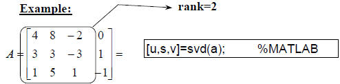
the number r is the rank of the matrix A.

The values σ_i are the square roots of the eigenvalues
of which we know are all because is
positive semi-definite.

The matrix V has columns consisting of the orthogonal
regular eigenvectors of matrix and matrix U has
columns consisting of regular eigenvectors of

The nonzero values together with the zero
values are called the singular values of
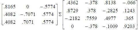
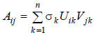
matrix A, and the expression

is called the singular value decomposition of A. It is not
a unique decomposition.

	two non-zero singular values

NOTE that the SVD is not computed using the eigenvectors
of the matrices. There are much more numerically stable
ways to compute it. We don't generally compute it "by
hand".

We will discuss four common applications of the SVD:

•  linear algebra operations

•  numerical stability analysis

•  matrix norm computations

•  uncertainty analysis

Performing some common linear algebra operations:

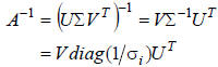
1. Matrix inverses: because the matrices U and V are
orthogonal (and may be made orthonormal), we can use
the SVD to compute a matrix inverse of a nonsingular
square matrix:

2. Solving simultaneous equations: Consider the
equation

One can show that the columns of U that correspond to
nonzero singular values σ_i form an orthonormal
basis for the range space of A. The columns of V
corresponding to nonzero singular values span the
null space of A.

If there exists a solution, or a number of them, the
formula

can be used to find x. If there are an infinite
number of solutions, this formula will give the
shortest solution x when we replace by zero
if (Giving the pseudoinverse solution!) Then
adding to x any linear combination of the columns of
V will give other solutions.

The same formula also applies when there are no
solutions, but we seek a "least-squared error"
approximate solution.

3. Approximation of matrices: From the definition of the
singular value decomposition, we can write the
expression:

This implies that we can "approximate" matrices by
throwing away some of the terms in this series: the
ones corresponding to excessively small singular
values. One could then store perhaps only a few
columns of U and V in order to recover A with
reasonable accuracy.

4. Rank determination: The SVD is the only numerically
stable way to determine the rank of a matrix!

The rank of a matrix is the number of nonzero singular
values. Of course, there will still be a judgement call
when some singular values are very small. Usually, a
"threshold" is chosen.

Numerical Stability Analysis:

Definition: Let f denote some mathematical operation to be
performed on a data quantity d. The operation is said to
be "well-conditioned" if f(d) is "near" f(d*) whenever d
is"near" d*. The definition of "nearness" depends on the
particular problem being solved.

An algorithm that performs f(d) is numerically stable if it
does not introduce any more sensitivity to perturbations
on the data than the mathematical operation itself does.
That is, if the algorithm itself is called f*, then f*(d) will be
"near" f(d*).

We say a matrix A is well-conditioned if computational
operations involving it are well-conditioned.

Definition: The condition number of a matrix is defined as
the ratio of the largest singular value to the smallest
singular value:

Singular matrices all have infinite condition numbers,
and the condition number for nonsingular matrices is a
measure of how "nearly singular" the matrix is.

As an example, if a matrix is "nearly" singular, then
computing its inverse might by numerically unstable
because the reciprocal of the singular values might
approach the machine's limit of precision.

The condition number also indicates, roughly, how
much an error in A or b will be magnified when
computing the solution to Ax=b.

Matrix Norm Computations:

Recall that the 2-norm ("Euclidean norm") of a matrix A
can be defined as:

or equivalently

One can also show that

(the largest singular value of matrix A)

There is another matrix norm that can be defined using
singular values: The Frobenius Norm

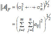
Matrix norms are best computed using singular values. The important area of study called robust control is heavily reliant on the computation of singular values for matrices.

Uncertainty Analysis:

An explanation of the use of singular values in
uncertainty analysis requires some background in
probability and random variables.

When, in a physical process, we are measuring a
quantity by using noisy, inaccurate sensors, we can
use singular value decompositions to determine the
uncertainty in our measurements along different
"directions."

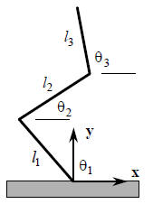
A good example (that also includes past topics from
linear systems) is from the study of robot kinematics:

Example: Consider the three-link planar robot, with the
joint coordinates shown.

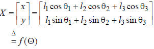
	The kinematic equations can be written in the following form:
	X is the Cartesian-coordinate location of the end of the robot given the joint-angle measurements.