Differential and Integral Calculus Review and Tutorial

1.3 Integral Calculus
Fast Facts:
1. Definition of a Definite Integral:
.
2. Definition of an Indefinite Integral:
3. The Indefinite Integral is an operator (it operates on functions).
4. In particular, the Indefinite Integral is the Accumulated Area Operator. The area is achieved by
summing many rectangles of length ∆x = (b − a)/N and height R f(a + i∆x). Thus, the units of
dx is the units of f(x) multiplied by the units of x.
5. The Indefinite Integral of any Elementary Function may or may not be an Elementary Function.

1.3.1 Some Integrals

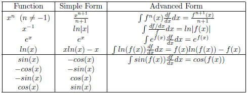
1.3.2 Techniques of Integration

Technique	When to Use
u-Substitution Integration by Parts Trigonometric Substitution Synthetic Division/Partial Fraction Series Solution	When it’s obvious or when you’re stuck. When you have a product of two functions, and you know the derivative of one and the integral of the other. When you have (a + x2) or (a − x2) terms. When you have a ratio of polynomials. When you stuck but realize a Taylor Series is easy to calculate.

As you may recall, the formula for integration by parts is
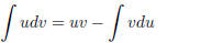(1.18)
A common mistake when using integration by parts on a definite integral is to forget to evaluate the uv term
with the integration limits.

1.3.3 Examples of Integration Techniques
Example (Advanced Forms)
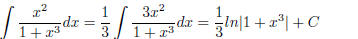(1.19)

Comment: The “Advanced Forms” involve what I call the “Hope Method.” You see a complicated function
and hope that the derivative of the inside of the equation is sitting on top. In this case it is. One is sometimes
taught to use u-Substitution here, but this integral should be done in your head. Notice how the integral
would be much harder if it is dx. That’s why it’s the Hope method, you hope that derivative is there!

Example (Advanced Forms)
(1.20)
Comment: One of my favorite integrals. By using the properties of the logarithm, we can make the derivative
show up by just multiplying by a constant. The integral could be done by integrating by parts, but it would
be longer and much less cool!!

Example (Integration by Parts)
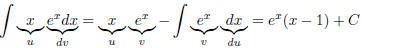(1.21)
Comment: You can see that if we had we would perform integration by parts n times, as the power
of the monomial decreases by 1 every time, but the exponential stays firm. It is a good idea to take the
derivative of your result to insure a correct answer. In this case the derivative is obtained by the product
rule: e^x(1) + (x − 1)e^x = xe^x as it must.

Example (Synthetic Division)

(1.22)
Comment: Use synthetic division on a rational function when the degree of the polynomial on top is greater
than or equal to that on the bottom. Some students haven’t done synthetic division in a while. It’s just
the same as long division you first learned in grade school. Unfortunately, you may have not done that in a
while either!

Example (Partial Fraction Expansion)
The integrand of
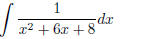 (1.23)
can be reduced by using a technique in ALGEBRA known as Partial Fraction Expansion. In particular, the
integrand can be rewritten
1
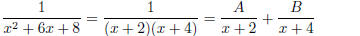(1.24)

Solving for A and B yields A = 1/2, B = −1/2. The solution is
(1.25)

Comment: For the integral of a fifth degree polynomial divided by a second degree polynomial, one would
use synthetic division first, and use Partial Fractions on the remaining integral. There is a technique where
the partial fractions coefficients can be determined by inspection.

Example (Series Solution)
To solve
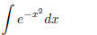(1.26)
we may note that the Taylor Series expansion for an exponential function is
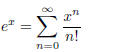(1.27)
Thus, the integral becomes
(1.28)
Comment: If you multiply our result by , we just found the Taylor Series expansion for erf(x).

Example (Trigonometric Substitution)
Find the area of a cirle. The equation of a circle is x² +y² = r². To find the area we will double the area of
the top half of the circle, which can be found be integration:
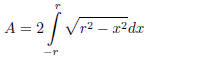(1.29)
Making the substitution x = rcos( ø ), it follows that dx = −rsin( ø )dø , and that
(1.30)
Comment: Trig sub gives expected answer.

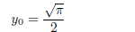
Example (Bonus Fun - Coordinate System Conversion)
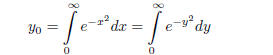(1.31)
Thus
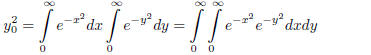(1.32)
Using a rectangular to polar conversion yields

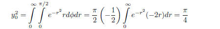
or
(1.34)
Comment: You can see why erf(x) has the normalized factor in front - it’s so that the area under the
erf(x) is 1. This solution is a fun little trick that only works when the integral is extended to infinity. In
general, though, if you see an integral whose limits are −∞ to ∞, look to see if the integrand is an odd
function (Hope Method). If it is, the integral is zero. Finally, notice that the area under the curve is finite,
but that the length of the curve is infinite. This deserves some thought. If you had such a box, it would
mean that you could fill the box with paint, but you would never have enough paint to paint the box!!
Interestingly, It is also possible to have figures which have infinite perimeter with a finite area. Fractals have
these properties.

1.4 Types and Methods of Solution
Since not all integrals have solutions in terms of Elementary functions, there are different types of solutions
that may be obtained. Not all of these have equal merit.
1. Exact Analytical Explicit Solutions. (Best)
2. Exact Analytical Implicit Solutions. (Good)
3. Series Solutions. (Not as good)
4. Numerical Solutions. (OK, if nothing else works)

Students should familiarize themselves with the following solution methods.
1. Analytical Methods (such as the “Techniques of Integration”, above).
2. Analytical and Numerical Solutions using Computer Algebra Systems (such as Maple).
3. Numerical Solutions using Spreadsheets.
4. Numerical Solutions using a programming language (such a C++).

As added motivation, students should be aware that
• These types and methods of solution apply to differential equations as well as integrals.
• Integrals are a special case of a differential equation.
• The laws of physics which apply to all of nature and devices created by man are governed by differential
equations, which, under many circumstances reduce to integrals.
• Many of the algorithms for numerical integration and solution to differential equations are available
(without charge) on the Internet (as is a host of related material). Try a web search for “Numerical
Recipes in C++.”

1.5 Applications of Calculus
There are very many applications of calculus. Below is a short table of functions and paramters of general
interest to the mathematical and scientific community.
 

Application	Formula
Area under curve Slope of curve Extremum of a curve (max, min, inflection pt.) Inflection point of a curve Arc Length Curvature (Radius) Average of a function RMS of a function
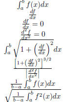Center of Mass Variance (Second Central Moment) Skewness (Third Central Moment) Kurtosis (Fourth Central Moment) Function Squared Norm
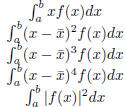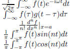
Fourier Transform Convolution Integral Taylor Coefficients Fourier Sine Series Fourier Cosine Series