Linear Equations

Chapter 1
1.1 Introduction

A linear equation (over the real numbers R) in the variables x₁ x₂, · · · , x_n is a
mathematical equation of the form

(1.1) 

with c and the coefficients a₁ · · · , a_n some arbitrary real numbers. If c = 0 then
the equation is homogeneous, otherwise it is inhomogeneous. A system of
linear equations is a set consisting of a finite number of linear equations, and a
solution to such a system is any set of specific values for the xi which make each
equation a true statement. When we have found all possible solutions we say,
appropriately enough, that the system has been solved. You may recall that either
substitution or elimination can be used to solve systems of linear equations:

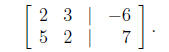
Example 1 Solve the following system of equations:

2x + 3y = −6
5x + 2y = 7.

We use elimination, say by multiplying the first equation by 5, the second by −2,

5(2x + 3y = −6) ----> 10x + 15y = −30
−2(5x + 2y = 7) ----> −10x − 4y = −14,

and then adding the transformed equations. This yields the single equation
11y = −44, so y = −44/11 = −4, and substituting this value for y back into either one
of the original equations, e.g. 2x + 3y = −6, gives us an equation in x, e.g.
2x + 3(−4) = −6. Thus x = (−6+12)/2 = 3, and we have found a unique solution
(x, y) = (3,−4) to the system of equations.

Some systems have more than one solution:

Example 2 Find all solutions to the system

2x − y = 5
8x − 4y = 20.

If we multiply the equation 2x − y = 5 by 4 and subtract the second equation, we
obtain the equation 0 = 0, in other words each equation has the same set of
solutions, so our elimination trick (which yields the intersection of the two solution
sets) gives us no new information. Using, e.g, the first equation, we may define the
solution set as {(x, 2x − 5) | x  R}.

And finally, the intersection of the solution sets may well be the empty set:

Example 3 Solve the system

2x − 3y = 1
4x − 6y = 6.

If we multiply the first equation by −2 and add the resulting equations, we obtain
the ridiculous statement 0 = 4, i.e. assuming there is a pair (x, y) common to each
solution set leads to a logical contradiction. Thus the system has no solution.

Classically, some of the earliest motivation for developing the theory of abstract
linear algebra came from calculus, specifically the study of differential equations.

Example 4 Find all real polynomials f(t) of degree less than 3 such that f(1) = 1,
f(3) = 3, and f0(2) = 3. (This is 1.1, #34 in your text.)

The generic polynomial of degree ≤2 has the form

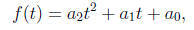
for arbitrary real numbers a₀, a₁, a₂. Thinking of these as variables, the given
information yields three linear equations:

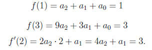
This time we employ substitution. The last equation says a₁ = 3 − 4a₂, and using
this in the other two equations yields the system

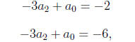
which clearly has no solution. Therefore the original system has no solution.
You may verify for yourself that if the initial conditions are changed to
“f(1) = 1, f(3) = 7, f0(2) = 3”, then the solutions are

Example 5 (1.1,#41.) Find a system of linear equations in x, y, z whose solution
set is {(6 + 5t, 4 + 3t, t + 2) | t Є R}.

One method is to substitute and eliminate t, e.g. using z = t + 2 we obtain
t = z − 2, and this reduces the equations

x = 6 + 5t
y = 4 + 3t

to the system

x = 6 + 5(z − 2) = 5z − 4
y = 4 + 3(z − 2) = 3z − 2,

i.e. the system

x − 5z = −4
y − 3z = −2
has the required properties. 2

Homework: Section 1.1, problems 1,6,7,13,18,22,30,32,36,38,40,44

1.2 Gauss-Jordan elimination

There is an algorithm, called Gauss-Jordan elimination, which solves a system of
linear equations, or shows that there are no solutions if that is the case. To begin,
we put the system of equations in augmented matrix form, e.g. the system from
Example 1 yields the augmented matrix

As in the example, we perform a series of row operations to the augmented matrix,
and put it in reduced row echelon form, which in the example gave us

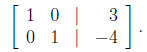
This is an augmented matrix whose correponding system of equations is

x = 3
y = −4,

and this provides the unique solution. The row operations we will use are
i) multiplying a given row by a nonzero scalar (real number).
ii) adding a multiple of one row to another row.
iii) interchanging two rows.

Reduced row echelon form provides us with the data needed to efficiently describe
the solution set to a given system of linear equations. Indeed, each nonzero row has
a leading 1, which corresponds to a dependent variable, i.e. the value of the
variable this 1 represents is determined uniquely by the other nonzero entries in
that row, which represent the constants in the linear equations and the coefficients
of the independent variables.

Example 6 Consider the following augmented matrix, which is in reduced row
echelon form:

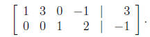
Suppose this matrix represents a system of linear equations in the variables
x₁, x₂, x₃, x₄. Which variables are dependent, and which are independent?

The corresponding system of equations is

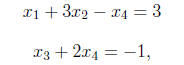
and from this we find that we may take x₃ and x₁ as dependent variables, and x₂, x₄
as independent. Note that we could also take x₂, x₃ as dependent and x₁, x₄ as
independent. This can be identified in the second column of the augmented matrix,
where there is a 3 in the first row, with all zeros below it. Each column of this sort
will give us another choice to make in the labeling of dependent and independent,
but it seems very convenient to adopt the convention that variables corresponding to
leading 1’s will always be labeled as dependent, and we do so now. With this
convention, we can write the solution set for Example 6 as

Example 7 (1.2, #9.) Use Gauss-Jordan elimination to solve the following system:

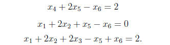
This system has the augmented matrix

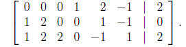
Following the technique in the text, we swap the first and third rows of the matrix,
obtaining

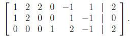
Then we multiply the first row by −1 and add this to the second row, obtaining

Now we divide the second row by −2, obtaining

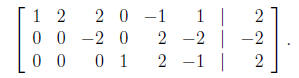
Finally, we multiply the second row by −2 and add this to the first row, obtaining

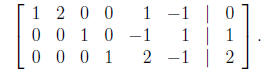
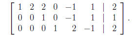
This augmented matrix is in reduced row echelon form, and the corresponding
system of equations is

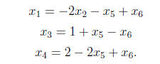
Thus there are three independent parameters, namely x₂, x₅, and x₆, and the
solution set can be represented as

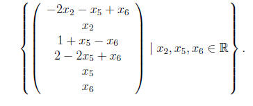
(This is given in vector notation, which will be discussed in the next section.)

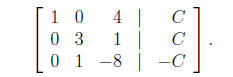
Example 8 (1.2,#49) Find the least positive integer C such that the system

2x + y = C
3y + z = C
x + 4z = C
has an integral solution, i.e. such that x, y, z are all integers.

We start with the augmented matrix

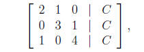
and after interchanging rows 1 and 3, and then adding −2 times the (new) first row
to the (new) third row, we obtain

Next we add −3 times row 3 to row 2, obtaining

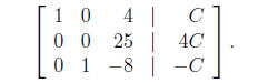
We then interchange rows 2 and 3

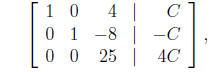
divide row 3 by 25

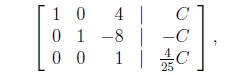
and then eliminate in the third column, obtaining

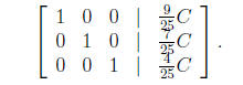
This gives the answer in terms of the free parameter C, i.e.

and we see that C = 25 is the least positive integer such that (x, y, z) Є Z³.

Homework: Section 1.2, problems 5,10,17,30,46,56,60

1.3 Matrix arithmetic

In general, a real n × m matrix is any rectangular array

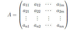
of real numbers, arranged in n rows and m columns. When we write A = (a_ij), we
mean that A is a matrix whose entry in the ith row, jth column is the real number
a_ij . Let Mat(n,m) denote the set of all real n × m matrices. We define addition in
Mat(n,m) entrywise, i.e. if A = (a_ij) and B = (b_ij) are arbitrary matrices in
Mat(n,m), then their sum is the n × m matrix A + B = (a_ij + b_ij).

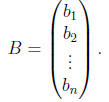
A 1 × n matrix is called a row vector

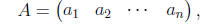
and an n × 1 matrix is a column vector

There is a kind of multiplication we can define between a row and column vector of
the same size. Taking A and B as above, we define

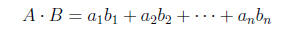
to be the dot product or scalar product of A and B.
If we have an A = (a_ij) in Mat(n,m) and a B = (b_ij) in Mat(m,k), then we can use
the dot product to define multiplication between A and B. To do this, just define
AB = (c_ij), where c_ij denotes the dot product of the ith row of A with the jth
column of B, i.e.

Note that AB Є Mat(n,k).
We write Mat_n(R) for the set Mat(n,n) of all square real matrices. We can both
add and multiply within this set, i.e. Mat_n(R) is closed under the addition and
multiplication operations defined above. This will be an important point later on.

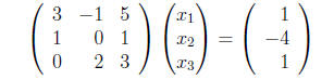
Example 9 Write the system

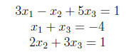
as a matrix equation.

This looks like

Just as with augmented matrices, we can perform row operations to put the
coefficient matrix of a matrix equation in reduced row echelon form, and we write
rref(A) to denote the reduced row echelon form of a matrix A. The number of
nonzero rows of rref(A) is called the rank of A, and we denote this number by
rank(A).
 

n the case n = m, the coefficient matrix is square, and we have the following

Theorem 1 Suppose A is the coefficient matrix for a system of n linear equations
in n variables. Then the system has a unique solution if, and only if, rank(A) = n.

Note that an n × n matrix A has rank n if and only if rref(A) has a 1 on each
diagonal entry and 0 in all the other entries. For example, if we reduce the
coefficient matrix

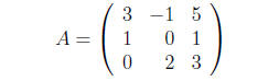
in Example 9, we obtain

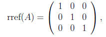
so we find that rank(A) = 3, and by Theorem 1 the system has a unique solution.

We call a system of linear equations consistent if there is at least one solution, and
inconsistent otherwise. If the system has n linear equations in m variables, and
n < m, then there cannot be a unique solution, i.e. there are not enough rows in the
augmented matrix to provide each variable with a leading 1, so some variables must
be independent if the system is consistent. Thus the system either has infinitely
many solutions, or is inconsistent and has no solution. It is easy to see that a
system is inconsistent if and only if the reduced row echelon form of its associated
augmented matrix contains a row of the form [ 0 0 · · · 0 | 1 ], representing
the unsatisfiable equation 0 = 1.

Homework: 1-4,9-12,16,19,22,27-30,36,37